Neural Network From Scratch: A Python Guide

You’re probably here for one of two reasons. Either you’ve used TensorFlow or PyTorch long enough to feel the abstraction getting in the way, or you’re evaluating AI for a product and want to know what’s happening under the hood before you trust it in production.

Building a neural network from scratch is one of the best ways to close that gap. It forces you to deal with matrix shapes, activation choices, initialization, and training dynamics instead of treating the model like a black box. That’s useful whether you write Python every day or lead a team integrating AI into a desktop, web, or mobile product.

It’s also a healthy reality check. A from-scratch implementation is excellent for learning. It is not automatically the right path for a production system that also needs version control for prompts, parameter governance, logging across AI providers, and visibility into cumulative spend. Those operational problems show up fast once AI leaves a notebook and enters a real application.

Why Build a Neural Network From Scratch

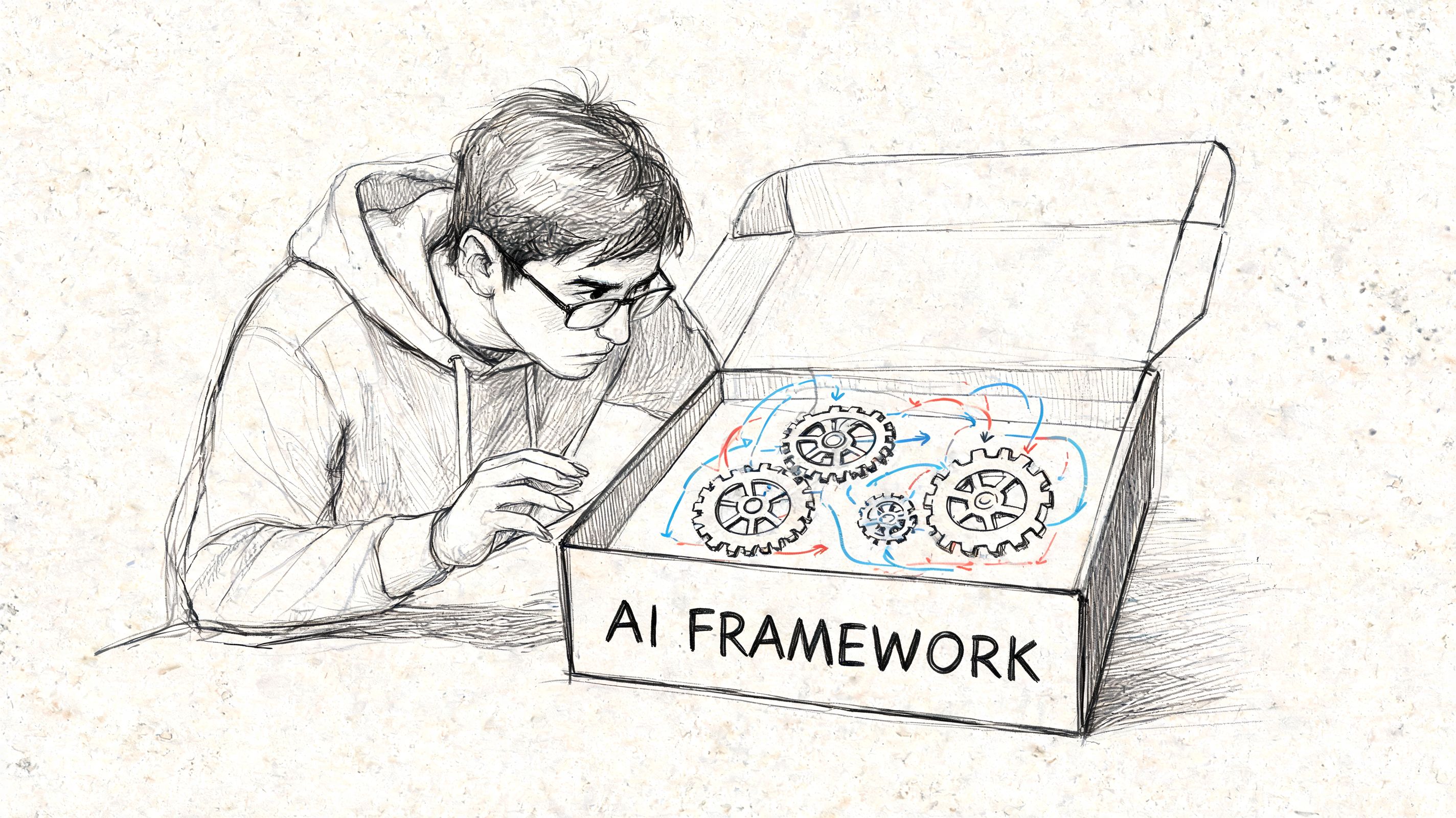
Frameworks are fantastic. They’re also very good at hiding the parts you most need to understand when training goes sideways.

A developer who builds a neural network from scratch learns what the framework usually handles for them. You stop saying “the model didn’t converge” and start asking better questions. Were the weights initialized badly? Did activations saturate? Did the learning rate push updates too far? Is the architecture too shallow for the pattern you want to learn, or too brittle for noisy business data?

That curiosity has deep roots. The basic architecture dates back to 1943, when Warren McCulloch and Walter Pitts modeled a simple neural network using electrical circuits. The first practical implementation didn’t arrive until 1958, when Frank Rosenblatt developed the Perceptron, as described in Stanford’s history of neural networks.

What you gain by doing it the hard way

A from-scratch build gives you three things that tutorials using high-level frameworks often don’t:

• Mechanical understanding: You see how inputs become outputs, then how errors become gradient updates.
• Debugging instincts: You learn to inspect activations, gradients, and loss curves instead of guessing.
• Architectural judgment: You get a much clearer sense of when a small custom network is enough and when the problem calls for established tooling.

For product teams, that judgment matters. If you’re exploring where AI belongs in a business workflow, this practical guide to implementing AI in business applications helps frame the broader integration question beyond the model itself.

Practical rule: Build from scratch to learn the machinery. Use mature platforms when reliability, observability, and team velocity matter more than educational value.

Where the exercise stops being enough

The limit of the exercise shows up the moment your model has to live inside software used by customers or internal teams. In a notebook, you can rerun training and move on. In production, you need guardrails.

That includes versioning model behavior, tracking changes to prompts and parameters, logging how integrated AI components behave over time, and watching cost as usage scales. Those aren’t “extra” concerns. They’re part of shipping AI responsibly.

So yes, it’s worth learning the internals. Just don’t confuse that with the full job.

The Blueprint of a Neural Network

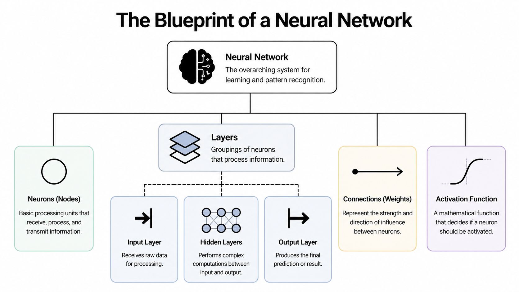
A neural network looks intimidating until you reduce it to a few moving parts. At its core, it’s just a chain of transformations applied to data.

A simple feedforward network has an input layer, one or more hidden layers, and an output layer. Each layer contains neurons, also called nodes. Neurons receive values, combine them using learned parameters, and pass the result forward.

The parts that actually matter

Here’s the mental model I use with new engineers.

Component	What it does	Why it matters
Input layer	Receives raw features	Defines what the model can “see”
Hidden layers	Transform inputs into richer representations	Let the network learn patterns beyond simple linear rules
Output layer	Produces the final prediction	Matches the task, such as classification or regression
Weights	Scale the influence of one neuron on another	Hold most of what the model learns
Biases	Shift activations before applying the nonlinearity	Help the model fit patterns more flexibly
Activation functions	Introduce non-linearity	Make the network capable of learning complex relationships

Without activation functions, stacked layers collapse into something much less interesting. You might have lots of parameters, but you still get a model that behaves like a linear transformation.

A practical analogy

Think of each neuron as a reviewer in a decision chain.

• The neuron receives several inputs.
• It gives each input a different level of importance through weights.
• It adds a small adjustment through a bias.
• It decides how strongly to respond through an activation function.

Two activation functions show up constantly in beginner implementations:

• Sigmoid: Useful for outputs that represent probabilities in binary classification.
• ReLU: A common hidden-layer choice because it’s simple and often easier to train.

A lot of beginner confusion comes from treating layers as magic. They’re not. They’re repeated blocks of weighted sums and non-linear decisions.

Design first, code second

Before writing NumPy, define the architecture in plain language.

Ask:

1. How many input features are there?
2. How many hidden layers do you want?
3. How many neurons should each hidden layer contain?
4. What shape should the output have?
5. Which activation function belongs in hidden layers and output?

That design step controls every matrix dimension you’ll create later. If your shapes are wrong, your implementation won’t just perform poorly. It won’t run.

For a first neural network from scratch, keep it small. One input layer, one or two hidden layers, and one output layer is enough to learn the mechanics without drowning in shape errors.

Coding the Forward Pass in Python

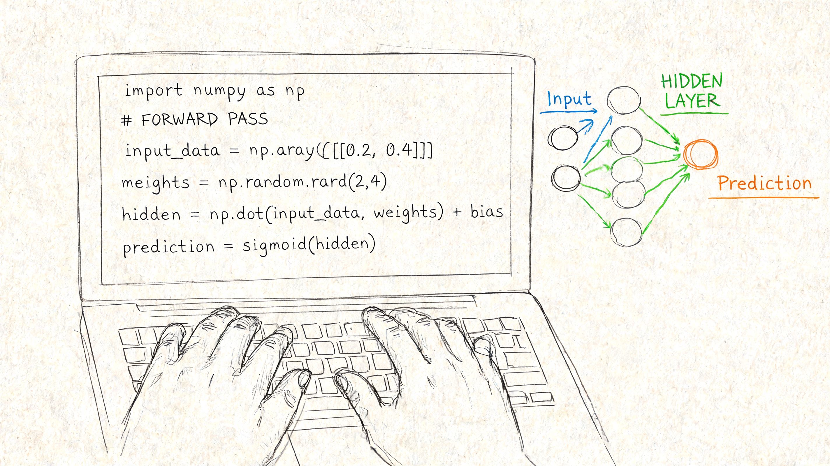
The forward pass is the part where your network makes a prediction. Input goes in, matrix multiplications happen, activation functions fire, and an output comes out.

If you’re coding this in Python, use NumPy and write it in a vectorized way. Don’t build the first version with many nested loops unless your real goal is learning how to make matrix code slow.

If you’re still setting up your environment, this comparison of Anaconda vs Python for machine learning work is a practical starting point.

Start with initialization, not optimism

Initialization is one of those details that feels minor until it ruins training. A practical pattern for the first weight matrix is:

np.random.randn(hidden_1, input_layer) * np.sqrt(1./hidden_1)

That specific scaling matters. According to the implementation notes in Neural Networks from Scratch, poorly scaled initialization can cause 30-50% slower convergence or prevent the network from learning meaningful representations at all.

Here’s a minimal structure:

import numpy as np

class SimpleNN:
    def __init__(self, input_size, hidden_size, output_size):
        self.W1 = np.random.randn(hidden_size, input_size) * np.sqrt(1. / hidden_size)
        self.b1 = np.zeros((hidden_size, 1))
        self.W2 = np.random.randn(output_size, hidden_size) * np.sqrt(1. / output_size)
        self.b2 = np.zeros((output_size, 1))

    def relu(self, z):
        return np.maximum(0, z)

    def sigmoid(self, z):
        return 1 / (1 + np.exp(-z))

Move data through the layers

The forward pass is just ordered arithmetic:

    def forward(self, X):
        self.Z1 = np.dot(self.W1, X) + self.b1
        self.A1 = self.relu(self.Z1)

        self.Z2 = np.dot(self.W2, self.A1) + self.b2
        self.A2 = self.sigmoid(self.Z2)

        return self.A2

A few implementation habits will save you time:

• Store intermediate values: You’ll need Z1, A1, and friends later during backpropagation.
• Check dimensions constantly: Shape mismatches are the most common bug in a first implementation.
• Use batches early: Even for a toy network, batch-shaped thinking leads to cleaner code.

What usually goes wrong

New builders often assume a bad output means the math is wrong. Sometimes it is. Often the architecture is fine and the initialization is the actual problem.

Common forward-pass failures include:

• Tiny activations everywhere: The signal shrinks and later layers learn slowly.
• Huge activations: Values explode, loss becomes unstable, and updates get erratic.
• Wrong output activation: A binary classification task with a poor output choice creates confusion fast.

If your network outputs nearly the same value for every input, inspect initialization before you redesign the whole model.

The forward pass should feel boring once it works. That’s a compliment. Predictable data flow is exactly what you want before adding the harder part.

The Art of Learning with Backpropagation

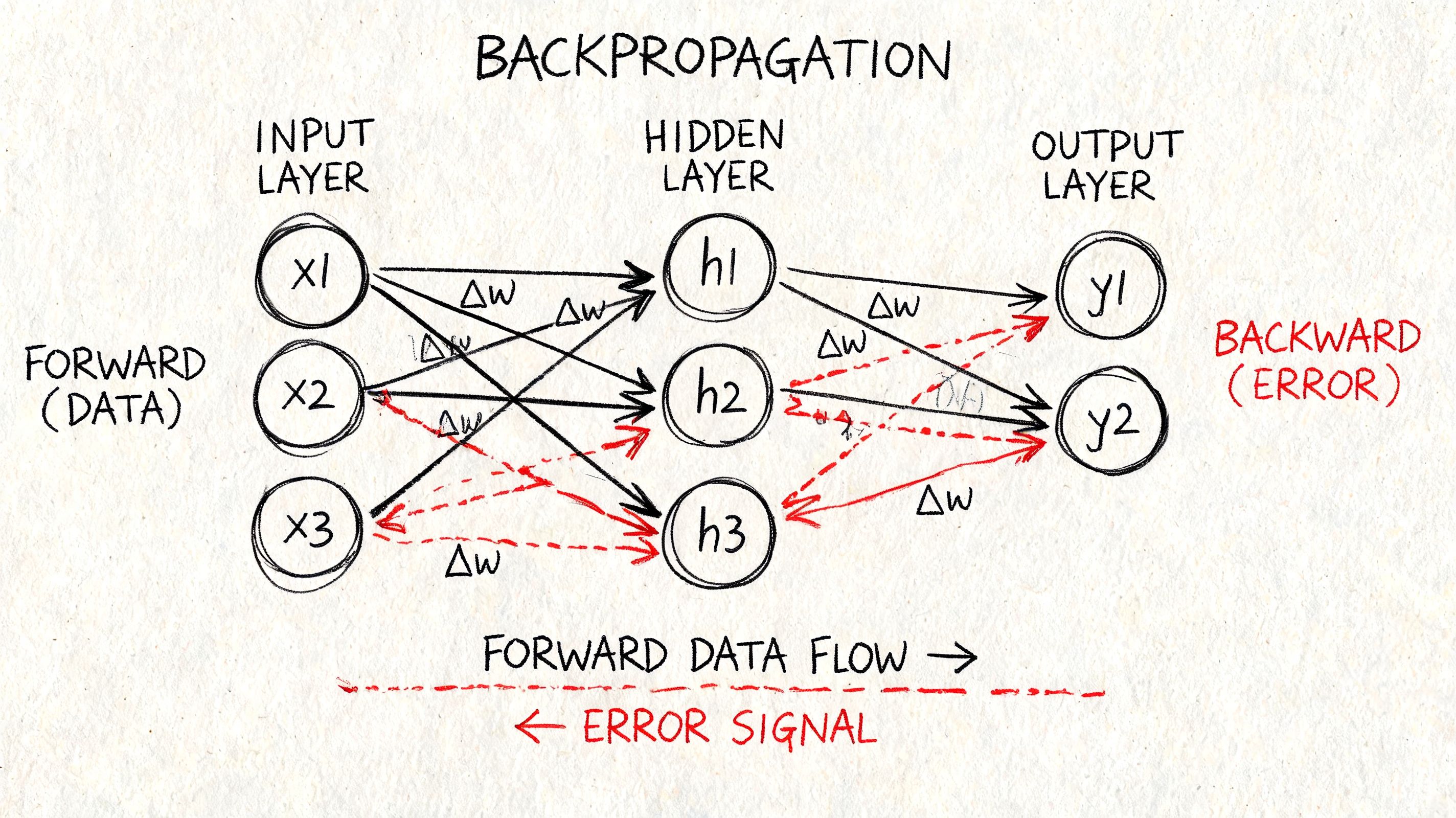
A network that only performs a forward pass is just doing arithmetic with random parameters. Learning begins when the model compares its prediction to the correct answer and adjusts itself.

That adjustment process is backpropagation. The intuitive version is simple. The model makes a mistake, measures how wrong it was, then sends responsibility backward through the network so each weight can change in the right direction.

Why backprop changed everything

Backpropagation became practical and influential when Rumelhart and Hinton popularized it in 1986. Its power showed up clearly in 1989, when Yann LeCun and colleagues used it to train a convolutional neural network to recognize handwritten ZIP codes. That training run took 3 full days, according to these Carnegie Mellon lecture slides on deep learning history.

That detail matters because it reminds people that elegant algorithms still live inside hardware limits. Training has always involved trade-offs between model complexity, compute, and patience.

Blame assignment in code

For a simple network, you compute the output error first, then propagate it backward.

def binary_cross_entropy(y_true, y_pred):
    eps = 1e-8
    return -np.mean(y_true * np.log(y_pred + eps) + (1 - y_true) * np.log(1 - y_pred + eps))

Now the backward pass:

def backward(self, X, Y, learning_rate=0.01):
    m = X.shape[1]

    dZ2 = self.A2 - Y
    dW2 = (1 / m) * np.dot(dZ2, self.A1.T)
    db2 = (1 / m) * np.sum(dZ2, axis=1, keepdims=True)

    dA1 = np.dot(self.W2.T, dZ2)
    dZ1 = dA1 * (self.Z1 > 0)
    dW1 = (1 / m) * np.dot(dZ1, X.T)
    db1 = (1 / m) * np.sum(dZ1, axis=1, keepdims=True)

    self.W2 -= learning_rate * dW2
    self.b2 -= learning_rate * db2
    self.W1 -= learning_rate * dW1
    self.b1 -= learning_rate * db1

What this code is really doing

The sequence is always the same:

1. Compute prediction error at the output.
2. Translate that error into gradients for output weights.
3. Pass the error backward into the hidden layer.
4. Compute hidden-layer gradients.
5. Update parameters.

That’s it. The elegance is in how the chain rule lets each layer reuse calculations from the layer after it.

Backprop isn’t magic. It’s bookkeeping for error.

The hard part is not memorizing the equations. The hard part is staying disciplined about shapes, derivative logic, and update order. One sign error, one transpose mistake, or one bad activation derivative is enough to freeze learning.

Training and Visualizing Your First Network

The first satisfying moment in a neural network from scratch project isn’t writing the class. It’s seeing loss move in the right direction.

Training combines the forward pass, loss calculation, backward pass, and parameter update into a loop that runs again and again. That repetition is the point. The model improves through many small corrections, not one dramatic insight.

A simple training loop

You can train on a toy problem such as XOR or a two-class dataset. The exact dataset matters less than being able to watch the network learn.

A basic loop looks like this:

losses = []

for epoch in range(1000):
    y_pred = nn.forward(X_train)
    loss = binary_cross_entropy(Y_train, y_pred)
    nn.backward(X_train, Y_train, learning_rate=0.1)
    losses.append(loss)

The training rhythm is always the same: forward pass → loss → backward pass → update. As noted in this R-based neural net walkthrough, this loop often needs to run across hundreds or thousands of epochs to reach strong accuracy.

What to visualize

Printing the loss every few epochs helps, but charts teach faster. Plot the training loss with Matplotlib so you can see whether learning is smooth, noisy, stalled, or diverging.

Useful visual checks include:

• Loss curve: Falling loss usually means the network is learning something.
• Decision boundary: For 2D toy data, this shows how the network separates classes.
• Prediction scatter: Overlay predicted labels on the data and inspect mistakes directly.

If you only look at one metric, make it the loss curve first. It exposes broken learning earlier than an accuracy number that looks fine for the wrong reasons.

The production trap

A beginner model can appear to work while still being useless in practice. The classic example is overfitting.

The same R tutorial notes a common failure mode where a model reaches 95%+ training accuracy but only 60-70% test accuracy, which makes it ineffective for production use. That’s why you should always compare training behavior with validation or test behavior, not just celebrate a high score on seen data.

A few signs you’re overfitting:

• Training loss keeps improving while validation performance gets worse.
• The model predicts the training set confidently but struggles on slightly new examples.
• Small architecture changes create big swings in test behavior.

A better habit than chasing accuracy

Treat the first training run as a diagnostic pass, not a final result. You’re checking whether the pipeline works, whether gradients flow, and whether the model can represent the pattern at all.

That mindset saves time. It also mirrors real product work, where a stable, inspectable training process is more valuable than one lucky run.

Advanced Techniques for Better Performance

A vanilla network is enough to learn the machinery. It’s rarely enough to handle messy data, unstable training, or a model that starts memorizing noise.

Practical engineering kicks in at this point. The goal isn’t to make the code look more advanced. The goal is to solve specific failures.

When training is slow or unstable

If learning crawls, jumps around, or gets stuck, try changing the training dynamics before redesigning the architecture.

A few reliable levers:

• Learning rate tuning: Too high and the loss bounces. Too low and the model barely moves.
• Better initialization: If activations or gradients behave poorly from the first batch, revisit your parameter scaling.
• Gradient clipping: Helpful when updates become erratic and the network diverges.

This is also where many developers graduate from plain gradient descent to optimizers such as Adam. The conceptual trade-off is straightforward. Simpler optimizers are easier to reason about. Adaptive optimizers often get you to a workable result faster.

When the model memorizes instead of generalizes

Overfitting usually needs a different response.

Try a mix of these:

• L2 regularization: Penalizes large weights and nudges the model toward simpler solutions.
• Dropout: Randomly disables part of the network during training, which discourages fragile co-dependencies.
• Early stopping: Stop training when validation loss stops improving, even if training loss still drops.

Here’s the key trade-off. Every regularization method adds friction to training. That friction is good when the model is memorizing noise and bad when the model already struggles to fit the signal.

The best “advanced technique” depends on the failure mode. Don’t reach for dropout when bad initialization is the real problem.

When architecture is the bottleneck

Sometimes the network is underpowered for the shape of the problem. Other times it’s too large for the amount of useful data you have. There isn’t a universal rule that says “more layers” or “more neurons” fixes things.

A practical decision pattern looks like this:

Symptom	Likely issue	First thing to try
Loss won’t decrease	Optimization or initialization problem	Check learning rate and initialization
Training improves, test degrades	Overfitting	Add regularization or stop earlier
Both train and test stay weak	Underfitting or poor features	Adjust architecture or input representation
Learning is erratic	Update instability	Lower learning rate or clip gradients

The useful lesson is that performance work is mostly diagnosis. Strong engineers don’t just know more techniques. They match the technique to the actual failure.

From Scratch to Production-Ready AI

A from-scratch build teaches the fundamentals. Production AI asks a different question. Can your system stay understandable, testable, secure, and affordable once real users depend on it?

That’s the line many teams cross without noticing. They start with a learning exercise, then bolt it into an internal tool, then connect it to customer data, then discover they now own an AI system that needs observability and governance.

The debugging gap is real

One of the least discussed problems in real-world AI work is diagnosing why a model fails. Tutorials are good at showing forward propagation and backpropagation. They’re much less helpful when the network trains poorly and nobody knows whether the root cause is architecture, initialization, alignment, data quality, or all four.

That gap shows up in a useful way in Simon Willison’s write-up of MIT CSAIL-related neural network learnability discussion, which notes that a 2025 MIT CSAIL result suggests network performance can depend more on its initial position in parameter space than on task-specific data. That’s a practical warning for teams modernizing legacy systems with AI. Sometimes the problem isn’t “we need more data.” Sometimes the model started in a bad place.

When to stop building from scratch

Stop when the educational return drops below the operational risk.

That usually happens when you need any combination of the following:

• Reliable deployment workflows: Repeatable training, evaluation, rollback, and release processes.
• Cross-system visibility: Logs that show what your AI components did, when, and why.
• Parameter and prompt control: A governed way to manage changing AI behavior across environments.
• Cost accountability: Clear tracking of cumulative AI spend across integrated services.

If your team is moving in that direction, it’s worth reading DataEngineeringCompanies.com's MLOps insights for a grounded view of the operational layer that sits around models.

The business decision

Many companies should shift from “can we code a model?” to “how should this AI capability live inside our software stack?” That broader decision includes model choice, integrations, monitoring, access patterns, and lifecycle management.

For teams weighing that next step, this overview of AI development services for custom software modernization is useful because it frames AI as part of an application architecture, not just a model in isolation.

The practical takeaway is simple. Build a neural network from scratch once. Maybe twice. You’ll become a better engineer for it. But don’t force a learning exercise to carry production responsibilities it was never meant to handle.

---

If you’re ready to move from experimentation to a maintainable AI product, Wonderment Apps can help. Their team works with organizations that need more than a model demo. They need AI integrated into real software, with the operational layer handled properly. That includes prompt vault versioning, parameter management for internal data access, unified logging across integrated AI systems, and cost tracking so leaders can see cumulative spend before it becomes a surprise.